Applications of TopoX to Equivariant Topological Networks
Studying the properties of message passing accross equivariant topological neural networks using the TopoX Suite
Introduction
Representation learning using Graph Neural Networks (GNNs) is a rapidly growing approach to complex tasks in chemistry
This blogpost aims to draw attention to Topological Deep Learning (TDL) by using the suite of Python packages TopoX
Higher-order networks and why topology is useful
Our regular and beloved graphs, as functional as they are, have a bound on the expressive power under message passing networks (MPN) that operate over them
In search of more expressive structures, the exploration of higher-dimensional topological spaces where higher-dimensional features, such as cliques, can be represented (and learned). Let’s start with what the space of a graph encodes. Let \(G = (V, E)\) be a graph. We can interpret it as encoding relationships between nodes \(u, v \in V\) as a tuple represented by an edge \((u, v) \in E\). What would relations between pairs of nodes and other pairs \((u,v) \rightarrow (x, y)\) or between pairs and triplets \((u, v, w) \rightarrow (x, y)\) would look like and how can we represent them? One space that allows for this kind of relationship is Simplicial Complexes. Extended graphs with features for higher dimensional structures are subjected to constraints. Luckily, the combinatorial definition of these spaces is more straightforward.
Simplicial Complex: What is it ?
An abstract simplicial complex (ASC) is the combinatorial expression of a non-empty set of simplices.
Concretly, let \(\mathcal{P}(S)\) be the powerset of \(S\) and let \(\mathcal{K} \subset \mathcal{P}(S)\), then \(\mathcal{K}\) is an ASC if for every \(X \in \mathcal{K}\) and every non-empty \(Y \subseteq X\) it holds that \(Y \in \mathcal{K}\). Also, we define the cardinality as \(\mid\mathcal{K}\mid = (\underset{X \in \mathcal{K}}{\operatorname{max} \mid X \mid }) - 1\), to be the highest cardinality of a simplex in an ASC minus 1. If the rank is \(r\), it holds \(\forall X \in \mathcal{K}: r \geq \mid X \mid\).
Click here for an example
Let \(S = \{0, 1, 2, 3\}\) and \(\mathcal{K} = \{0, 1, 2, 3, \{0, 1\}, \{1, 2\}, \{0, 2\}, \{0, 1, 2\}\}\) where we could pick an arbitrary element \(X = \{0, 1, 2\}\) and check that \(\forall Y \subseteq X: Y \in \mathcal{K}\). Meaning that for any possible subset \(Y\) in \(X\), \(Y\) is contained in \(\mathcal{K}\). In this case, the set \(\mathcal{K}\) is an ASC.
Geometric realization
Although an ASC is a purely combinatorial object, it always entails a geometric realization. A Simplicial Complex is the geometric realization of an ASC, constructed out of the underlying geometric points in \(\mathcal{K}\). Thus, Simplicial Complex of dimension $1$ is equivalent to a geometric graph (can you see why ?).
The procedure of transforming a structure to a topological domain is commonly called lifting. Thus, lifting can be from point clouds to graphs, graphs to simplicial complexes, or other pairs of domains, given that the properties of the target domain mentioned before hold.
Click here to see the ASC corresponding to Figure 1
As an example, let \(S = \{1, 2, 3, 4, 5, 6, 7\}\) and \(\mathcal{K} = \{ \{5, 6, 7\}, \{5, 6\}, \{5, 7\}, \{6, 7\}, \cdot \cdot \cdot, \{1,2\},\{2, 3\}, \cdot \cdot \cdot, \{1\}, \{2\}, \{3\}, \cdot \cdot \cdot\}\)

Clique Complex
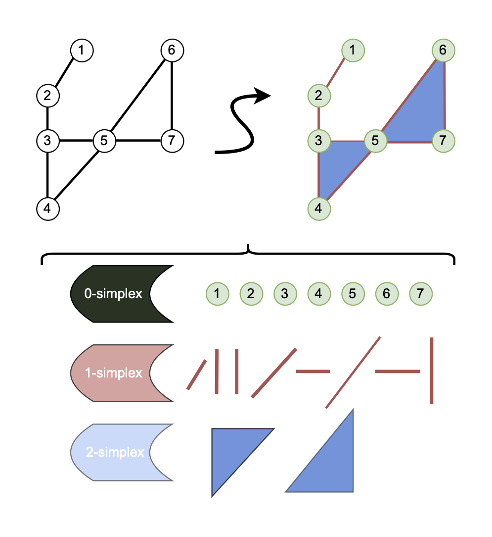
Of the plethora of spaces, a relatively simple and intuitive one is the Clique Complex shown at the top left of Figure 1. To describe the Clique Complex we need to formally define a clique, something we skipped over before.
Click here for a formal definition of clique
Given a graph \(G = (V, E)\), a clique \(C \subseteq V\), is an induced graph on \(G\) such that \(C\) is complete. In other words, there is an edge between every pair of vertices in \(C\).
The Clique Complex is a Simplicial Complex of rank \(1\). Each clique will become an \(r\)-simplex depending on the cardinality of \(C\) such that \(r=\mid C \mid-1\). The number of cliques grows exponentially, and the problem of finding all the cliques is complex. For this reason, the naive time complexity of this lift is \(\mathcal{O}(3^{n/3})\)
Vietoris-Ripps Complex
The Vietoris-Rips complex is a common way to form a topological space efficiently. The time complexity for generating the procedure depends on the parameter \(\delta\) and the number of points \(n\) given by \(\mathcal{O}(n^{r+1})\), where \(\delta\) is the diameter of the balls grown around points to calculate relationships. This space is equivalent to a Clique Complex in a geometric graph. Below, you can see a visualization of the lifting process with varying values of \(\delta\). The points are 0-simplex , the lines are 1-simplex and the triangles are 2-simplex . The growing ball is the disk relating to the \(\delta\) parameter.
GNNs and E(n) Equivariant GNNs
GNNs come in many flavors, but to be concise, we will focus on the Message Passing Networks where messages are passed among neighborhoods, which update the node’s representation. At a given number of passes, we will take the node representations and perform classification or regression tasks or pool them to perform the task on the whole graph. Next, we will introduce the remainder of the MPN framework and equivariant GNNs.
Good ol’ message passing
Let \(G = (V,E)\) be a graph consisting of nodes \(V\) and edges \(E\). Then let each node \(v_i \in V\) and edge \(e_{ij} \in E\) have an associated node feature \(\mathbf{f}_i \in \mathbb{R}^{c_n}\) and edge feature \(a_{ij} \in \mathbb{R}^{c_e}\), with dimensionality \(c_n, c_e \in \mathbb{N}_{>0}\). Then, we define a message passing layer as:
\[\begin{equation}\label{compute_message} \mathbf{m}_{i j}=\phi_m\left(\mathbf{h}_i^l, \mathbf{h}_j^l, \mathbf{a}_{i j}\right) \end{equation}\]\(\begin{equation}\label{aggregate_messages} \mathbf{m}_i=\underset{j \in \mathcal{N}(i)}{\operatorname{Agg}} \mathbf{m}_{i j} \end{equation}\) \(\begin{equation}\label{update_hidden} \mathbf{h}_i^{l+1}=\phi_h\left(\mathbf{h}_i^l, \mathbf{m}_i\right) \end{equation}\)
E(n) equivariant GNN
Using inductive biases to steer the training of GNNs towards a particular domain is common. There is a specific class of problems where symmetries are an intrinsic part of their representation. Examples of these are 3D molecular structures and N-body systems. To enhance the learning procedure, we restrict the families of learned functions by guaranteeing equivariance with the action of a transformation from a particular symmetry group. Of of those groups is the \(E(n)\) group, which encodes rotation, translation, reflection and scaling ( Euclidean group of dimension \(n\) ).
Tasks: QM9 and N-Body
QM9 is a dataset of 134K small molecules (up to \(9\) atoms without counting hydrogen) with \(19\) regression tasks representing the molecule’s properties. Each atom has a set of features and a position in 3D space. Pytorch geometric makes this dataset available in a convenient graph representation. The N-body problem extends the “Charged particle N-body system” to 3D where \(5\) particles have a positive and negative charge, position, and velocity. Then, the prediction is used to estimate the particle’s position after the steps of \(n\).
Equivariance and Invariance
Invariance is when an object or set of objects remain the same after a transformation. In contrast, equivariance is a symmetry concerning a function and a transformation. At first glance, these definitions are complicated to picture; however, with some group theory, they will become more apparent.
Let \(G\) be a group and let \(X\), \(Y\) be sets on which \(G\) acts. A function \(f: X \rightarrow Y\) is called equivariant with respect to \(G\) if it commutes with the group action. Equation \ref{eq:equi} expresses this notion formally.
\[\begin{equation}\label{eq:equi} f(g \cdot x)=g \cdot f(x) \end{equation}\]Conversly, Equation \ref{eq:inv} shows that invariance is when the application of the transformation \(g \in G\) does not affect the output of the map \(f\),
\[\begin{equation}\label{eq:inv} f(g \cdot x)=f(x) \end{equation}\]Do invariances hold in GNNs ?
Equation \ref{eq:msg_eq} comes to replace Equation \ref{compute_message} with our invariant function. To make the network equivariant, we introduce feature vector \(x\), which contains the positional coordinates in Euclidean space. Equation \ref{eq:pos_update} refers to the update in the position embedding of the node. The proof that with this condition, equivariance holds can be found in
Message Passing Simplicial Networks (MPSN)
In
Higher-order neighborhoods
We establish some definitions to define proximity relations, such as graph adjacencies in \(r\)-simplex. We will work with only two types of adjacencies as they have proven to be as expressive as using all of them. First, let \(\sigma\) and \(\tau\) be two simplices, we say that \(\tau\) is on the bound of \(\sigma\) or \(\tau \prec \sigma\) if :
- \[\tau \subset \sigma\]
- \[\nexists \delta: \tau \subset \delta \subset \sigma\]
Equation \ref{eq:bound_adj} referes to the relation between a \(r\)-simplex and the \((r-1)\)-simplex that compose it. Equation \ref{eq:bound_up} referes to the relationship between \((r-1)\)-simplex and other \((r-1)\)-simplex that are a part of a higher \(r\)-simplex. They are also referred to as cofaces in the literature
Equivariant relations
We will make use of previous definitions in the following small section. Recall that we showed that we can choose any \(f\) such that when applying to a certain class of objects invariant, it is invariant with respect to the group action of any \(g \in G\) for \(G = E(n)\) in this case. The authors of the paper choose four types of message passing. Each of these will have a set of geometric features depending on \(f\). In general \(p_i\) and \(p_j\) mean a shared point, \(a\) and \(b\) are points not shared.
| Num | \(\bullet \rightarrow \bullet\) | \(\bullet \rightarrow |\) | \(| \rightarrow |\) | \(| \rightarrow \triangle\) |
|---|---|---|---|---|
| 1 | \(\parallel x_{\mathbf{a}} - x_{\mathbf{b}}\parallel\) | \(\parallel x_{\mathbf{p}_i} - x_{\mathbf{b}}\parallel\) | \(\parallel x_{\mathbf{p}_i} - x_{\mathbf{a}}\parallel\) | \(\parallel x_{\mathbf{p}_i} - x_{\mathbf{a}}\parallel\) |
| 2 | 0 | 0 | \(\parallel x_{\mathbf{p}_i} - x_{\mathbf{b}}\parallel\) | \(\parallel x_{\mathbf{p}_i} - x_{\mathbf{a}}\parallel\) |
| 3 | 0 | \(\parallel x_{\mathbf{p}_i} - x_{\mathbf{b}}\parallel\) | \(\parallel x_{\mathbf{a}} - x_{\mathbf{b}}\parallel\) | \(V(S_2)\) |
| 4 | - | - | \(\parallel x_{\mathbf{p}_i} - x_{\mathbf{a}}\parallel\) | \(\parallel x_{\mathbf{p}_i} - x_{\mathbf{a}}\parallel\) |
| 5 | - | - | \(\parallel x_{\mathbf{p}_i} - x_{\mathbf{b}}\parallel\) | \(\angle \mathbf{p}_i + \angle \mathbf{p}_j\) |
| 6 | - | - | \(\angle \mathbf{p}_i\) | \(\angle \mathbf{a}\) |

Does it work on higher-order networks ?
Using the previous definitions of neighborhoods,
Finally, they define a graph embedding as Equation \ref{eq:agg_simp} where the simplices \(\mathcal{K}\) of each dimension \(r\) will be aggregated, and the final embedding of the complex will be the concatenation of the embedding of each dimension.
\[\begin{equation}\label{eq:agg_simp} h_{\mathcal{K}} = \bigoplus_{i=0}^{r} \underset{\sigma \in \mathcal{K}, |\sigma|=i+1}{\operatorname{Agg}} h_\sigma \end{equation}\]The new standard: TopoX
TopoX is a suite of Python packages that aims to fill the need for accessible and open-source software libraries to handle earning in higher-order domains. In the words of the team behind it, one of its goals is:
facilitate research in topological domains by providing foundational code to understand concepts and offer a platform to disseminate algorithms
Given the rapid theoretical advancements in TDL, the need for a solid experimental playground is clear. Many of the development setups would benefit in terms of development efficacy and replication capabilities by sharing a set of standards and practices. TopoX is compromised of four modules: TopoModelX, TopoNetX, TopoEmbbedX and TopoBenchmarkX
- TopoModelX: Variety of models based on higher-order message passing built on top of Pytorch
- TopoNetX: Similar to NetworkX it provides utilities to handle nodes, edge, higher-order cells and the calculation of adjacencies, incidences and hodge laplacians over complexes
- TopoEmbeddX: Embedding of topological domains in euclidean domains
- TopoBenchmarkX : Addition of datasets, transform such as lifts and new deep learning models
Next, we illustrate the development process and reproduction of
1. Building structure
We are first concerned with the lifting of our initial graph or set of points. To perform that task, we will make use of GHUDI forward that looks like this.
    def forward(self, data: torch_geometric.data.Data) -> torch_geometric.data.Data:
        r"""Applies the full lifting (topology + features) to the input data.

        Parameters
        ----------
        data : torch_geometric.data.Data
            The input data to be lifted.

        Returns
        -------
        torch_geometric.data.Data
            The lifted data.
        """
        initial_data = data.to_dict()
        lifted_topology = self.lift_topology(data)
        lifted_topology = self.feature_lifting(lifted_topology)
        return torch_geometric.data.Data(**initial_data, **lifted_topology)
In essence, we only need to define a subclass of the source and target domain of our choice (in this case Graph2SimplicialLifting) and override the lift_topology method and the apply feature lifting.
 def lift_topology(self, data: torch_geometric.data.Data) -> dict:
        simplicial_complex = rips_lift(data, self.complex_dim, self.delta)

        feature_dict = {}
        for i, node in enumerate(data.x):
            feature_dict[i] = node

        simplicial_complex.set_simplex_attributes(feature_dict, name='features')

        return self._get_lifted_topology(simplicial_complex, data)
In this case, we introduced rips_lift, which is going to do the actual computation of the lift, and _get_lifted_topology which will transform our SimplicialComplexinto a Pytorch Data object.
def rips_lift(graph: torch_geometric.data.Data, dim: int, dis: float,
                    fc_nodes: bool = True) -> SimplicialComplex:
    x_0, pos = graph.x, graph.pos

    points = [pos[i].tolist() for i in range(pos.shape[0])]

    rips_complex = gudhi.RipsComplex(points=points, max_edge_length=dis)
    simplex_tree: SimplexTree  = rips_complex.create_simplex_tree(max_dimension=dim)

    if fc_nodes:
        nodes = [i for i in range(x_0.shape[0])]
        for edge in combinations(nodes, 2):
            simplex_tree.insert(edge)

    return SimplicialComplex.from_gudhi(simplex_tree)
Note that optionally, nodes are fully connected, per the implementation of _lifted_topology, we build the matrix representation of our complex. The library provides the get_complex_connectivityand constructs the connectivity matrices.
    def _get_lifted_topology(
        self, simplicial_complex: SimplicialComplex, graph: nx.Graph
    ) -> dict:
        lifted_topology = get_complex_connectivity(
            simplicial_complex, self.complex_dim, signed=self.signed
        )

        for r in range(0, simplicial_complex.dim+1):
            # Convert to edge_index format
            lifted_topology[f'adjacency_{r}'] =
            lifted_topology[f'adjacency_{r}'].to_dense().nonzero().t().contiguous()

            lifted_topology[f'incidence_{r}'] =
            lifted_topology[f'incidence_{r}'].to_dense().nonzero().t().contiguous()


        for r in range(0, simplicial_complex.dim+1):
            # Returns the list of `r`-simplex as `r`-tuples and convert to tensor
            lifted_topology[f'x_idx_{r}'] =
            torch.tensor(simplicial_complex.skeleton(r), dtype=torch.int)

        lifted_topology["x_0"] = torch.stack(
            list(simplicial_complex.get_simplex_attributes("features", 0).values())
        )

        return lifted_topology
Note that we transform the adjacency and incidence matrices to their edge_index form by using nonzero().t().contigous(). This transformation is to be able to perform mini-batching during training.
2. Giving meaning to structure
Now that we have a higher-order topological space, we are missing only one thing. What should the embeddings of the \(r\)-simplex higher than \(0\) be ?
There is still the question of what a good feature-lifting technique constitutes and what information it should take from the underlying representation. Authors in
Formally, if \(\mid \sigma \mid > 1\), then:
\[f(\sigma) = mean(\{ f(\tau) \; | \; \tau \prec \sigma \wedge \nexists \delta: \tau \prec \delta \prec \sigma \})\]Click here for an example
Let \(\sigma = \{a, b, c\}\) be a simplex where \(a,b,c \in R^d\) and denote the feature embedding of \(\sigma\) with \(f(\sigma)\). Then, given those simplices on the boundary are given by the powerset such that \(\tau_1 = \{a, b\}, \tau_2=\{b, c\}, \tau_3=\{a, c\}\) and \(\forall i \in \{1, 2, 3\}: \tau_i \prec \sigma\) and \(\delta_1=\{a\}, \delta_2=\{b\}\) we have that \(f(\tau_1) = mean(f(\delta_1), f(\delta_2))\) and \(f(\sigma) = mean(f(\tau_1), f(\tau_2), f(\tau_3))\).
3. The Model
On the model side, the most interesting addition is by TopoModelX and the Conv class. This class represents the convolution operator on the graph, which is necessary for aggregating messages over the neighborhood. We show our implementation of the Conv class to allow equivariant information to pass inside the messages. Everything else is standard Pytorch (unless we use one of the provided models)
    def forward(self, x_source, edge_index, x_weights, x_target=None) -> torch.Tensor:
        # Construct the edge index tensor of size (2, n_boundaries)
        # x_weights is indexed with send_idx because there might be more relationships
        # than r-cells, in that case the weights are not aligned
        x_message = torch.cat((x_source[send_idx], x_target[recv_idx], x_weights), dim=1)

        if self.weight_1 is not None:
            x_message = torch.mm(x_message, self.weight_1)
            if self.biases_1 is not None:
                x_message += self.biases_1
            x_message = self.update(x_message)
        if self.weight_2 is not None:
            x_message = torch.mm(x_message, self.weight_2)
            if self.biases_2 is not None:
                x_message += self.biases_2
            x_message = self.update(x_message)
        if self.weight_3 is not None:
            x_message_weights = torch.mm(x_message, self.weight_3)
            if self.biases_3 is not None:
                x_message_weights += self.biases_3
            x_message_weights = torch.nn.functional.sigmoid(x_message_weights)
        else:
            x_message_weights = torch.ones_like(x_message)

        # Weight the message by the learned weights
        x_message = x_message * x_message_weights

        return x_message
4. Application
Now, on to the most important part. We con now very easily execute our model. To load our dataset, it is straightforward
dataset_name = "manual_dataset"
dataset_config = load_dataset_config(dataset_name)
loader = GraphLoader(dataset_config)
dataset = loader.load()
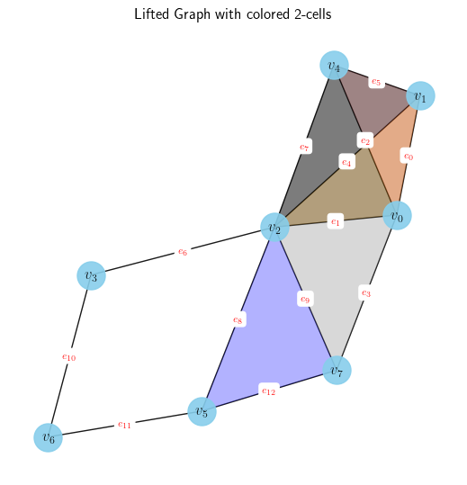
We can also visualize the information in point cloud, simplicial complex, or cell complex domains. Figure 3 is one such of test Simplicial Complex
describe_data(dataset)

After setting the configurations, using a lifting procedure is as easy as defining it’s name.
# Define transformation type and id
transform_type = "liftings"
# If the transform is a topological lifting,
it should include both the type of the lifting and the identifier
transform_id = "graph2simplicial/empsn_lifting"

# Read yaml file
transform_config = {
    "lifting": load_transform_config(transform_type, transform_id)
    # other transforms (e.g. data manipulations, feature liftings) can be added here
}
lifted_dataset = PreProcessor(dataset, transform_config, loader.data_dir)
Finally, we load our model and execute it.
from modules.models.simplicial.empsn import EMPSNModel

model_type = "simplicial"
model_id = "empsn"
model_config = load_model_config(model_type, model_id)

model = EMPSNModel(model_config, dataset_config)oy_hat = model(lifted_dataset.get(0))
y_hat = model(lifted_dataset.get(0))
Experiments
We performed experiments with the implementation in the TopoX framework. Additionally, we vectorized and improved the following sections: 1) the lifting procedure now results in a smaller file size, and the vectorization of the feature embeddings and adjacency/incidence matrix calculation with the help of TopoX is faster; 2) we organized the computation of the invariants, and further vectorized some operations.
Next, we present a comparison of the lifting times of the whole QM9 dataset, the size of the pre-processed file (after lifting), and the time it takes to run a forward pass.
Lifting times
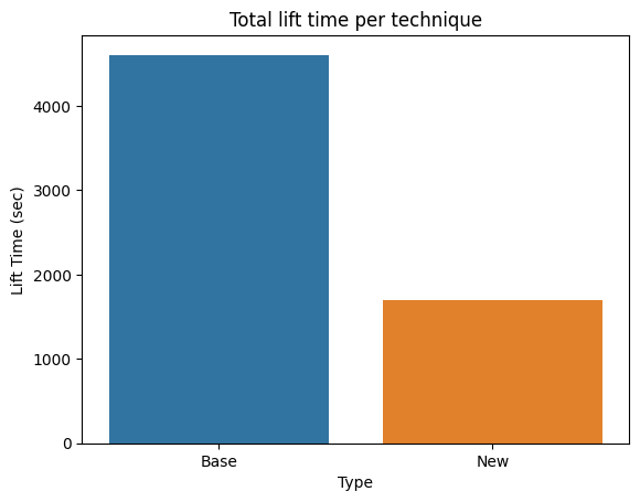
The lifting procedure has two challenging areas optimized: 1) calculation of the adjacency and incidence relationships for which we rely on TopoX, and 2) feature lifting, which we manually optimized. We brought down the lifting time from about 1.5 hours to about 28 minutes on the same hardware. Next, we show the lifting time of each graph in the dataset and compare the total lifting time. We see that our optimization could be much faster on the heavier graphs. However, there is a set that is reduced to the baseline.


File size
We observed a reduction in the size of the preprocessed dataset after the lifting procedure. This behavior is due to the way incidences and adjacencies are stored. Instead of having the invariance information directly, we can store the relationships, such as boundaries, upper adjacencies, and embeddings, which makes it enough. We could have also stored these as sparse tensors; however, handling the mini-batching proved cumbersome on that representation. Ultimately, we reduced the size from 8.7GB to 6.3 GB.
Forward pass
One of these models’ bottlenecks is the time they take to train for an epoch. The original version took close to 70 hours in the cluster we had access to. Some of this time is related to the number of messages passing and some to calculating the invariances, which must be done each forward pass. We managed to optimize this calculation and thus speed up the execution of the model almost ten-fold. These results are calculated over the forward on a batch size of \(96\), as per the original implementation, and take into account \(96\) batches.

Replication of results
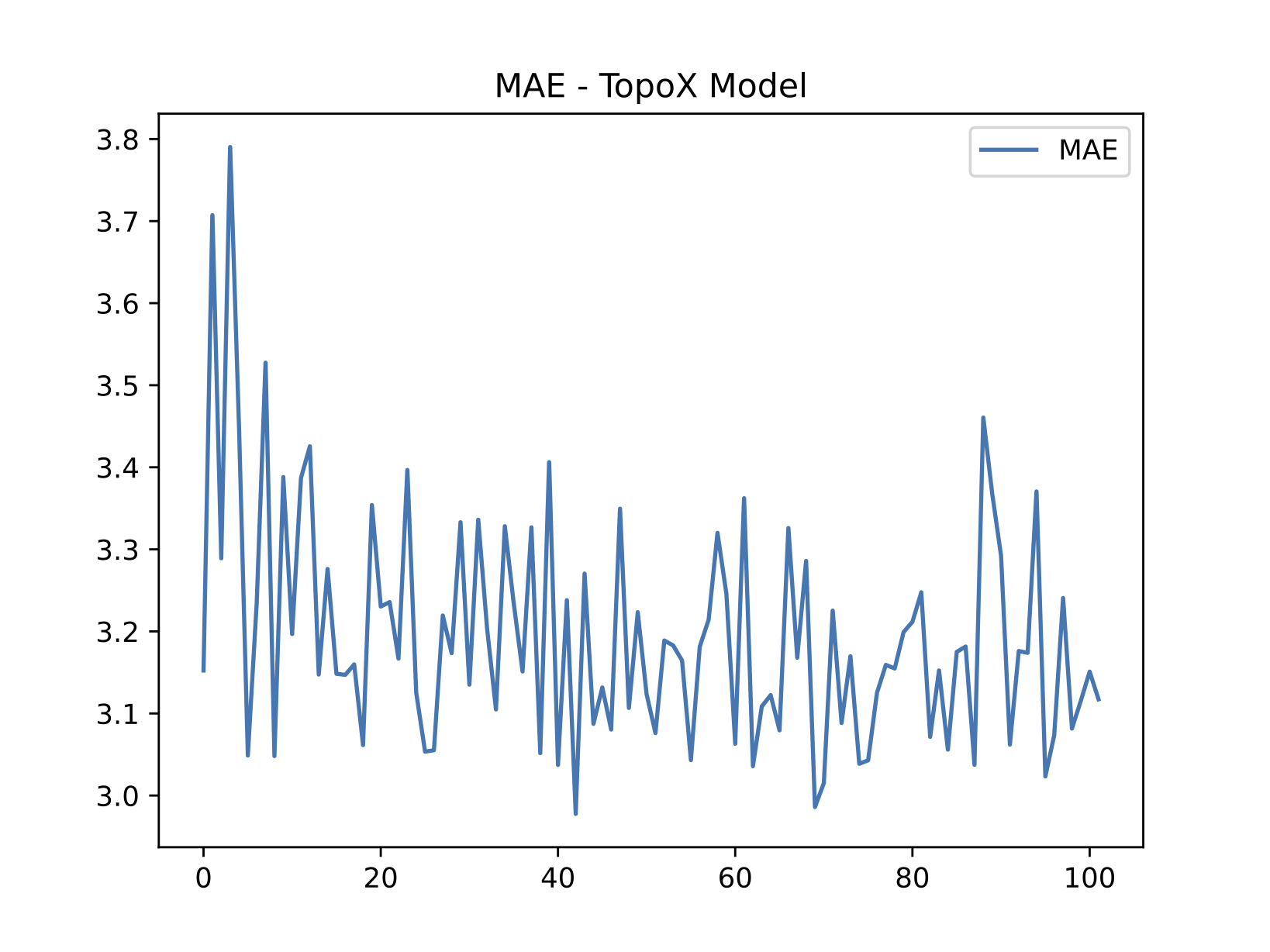
On the side of replication, we executed the original, publicly available code shown in Figure 4. Figure 5 compares our implementation and execution using the same hyperparameters set in the code. Due to computing constraints, we could not run experiments on the number of epochs set in the original codebase. For that reason, we report on two particular experiments:
- Execution of the original implementation up to epoch ~700.

- Execution of our implementation up to epoch ~100.

Our scores are not near SOTA or the reported scores in the original work. Nevertheless, thanks to the optimizations mentioned above, we were able to execute different tests during the procedure for a reduced number of epochs. Varying batch sizes and learning rates, as well as using other common weight initialization techniques, did not improve the results.
Conclusions
In this post, we superficially introduced the field of topological deep learning and placed it in the field of graph neural networks. Additionally, we investigated the novel development suite for Topological Deep Learning (TopoX) and how it can be used to tackle a particular problem. We review concepts in geometric deep learning and show why they work and how we can leverage topological representations to better learn in message-passing networks. Using the unified TopoX framework allows for ease of development and standardization regarding reproducibility. Additionally, optimization for computationally heavy procedures such as the ones inherent to TDL is more straightforward. Additionally, we replicate the work of