Grasping Graphormer : Assessing Transformer Performance for Graph Representation
A first-principles blog post to understand the Graphormer.
Introduction
The Transformer architecture has revolutionized sequence modelling. Its versatility is demonstrated by its application in various domains, from natural language processing to computer vision to even reinforcement learning. With its strong ability to learn rich representations across domains, it seems natural that the power of the transformer can be adapted to graphs.
The main challenge with applying a transformer to graph data is that there is no obvious sequence-based representation of graphs. Graphs are commonly represented by adjacency matrices or lists, which lack inherent order and are thus unsuitable for transformers.
The primary reason for finding a sequence-based representation of a graph is to combine the advantages of a transformer (such as its high scalability) with the ability of graphs to capture non-sequential and multidimensional relationships. Graph Neural Networks (GNNs) employ various constraints during training, such as enforcing valency limits when generating molecules. However, choosing such constraints may not be as straightforward for other problems. With Graphormer, we can apply these very constraints in a simpler manner, analogous to applying a causal mask in a transformer. This can also aid in discovering newer ways to apply constraints in GNNs by presenting existing concepts in an intuitive manner.
Graphormer introduces Centrality Encoding to capture the node importance, Spatial Encoding to capture the structural relations, and Edge Encoding to capture the edge features. In addition to this, Graphormer makes other architectures easier to implement by making various existing architecture special cases of Graphormer, with the performance to boot.
Preliminaries
-
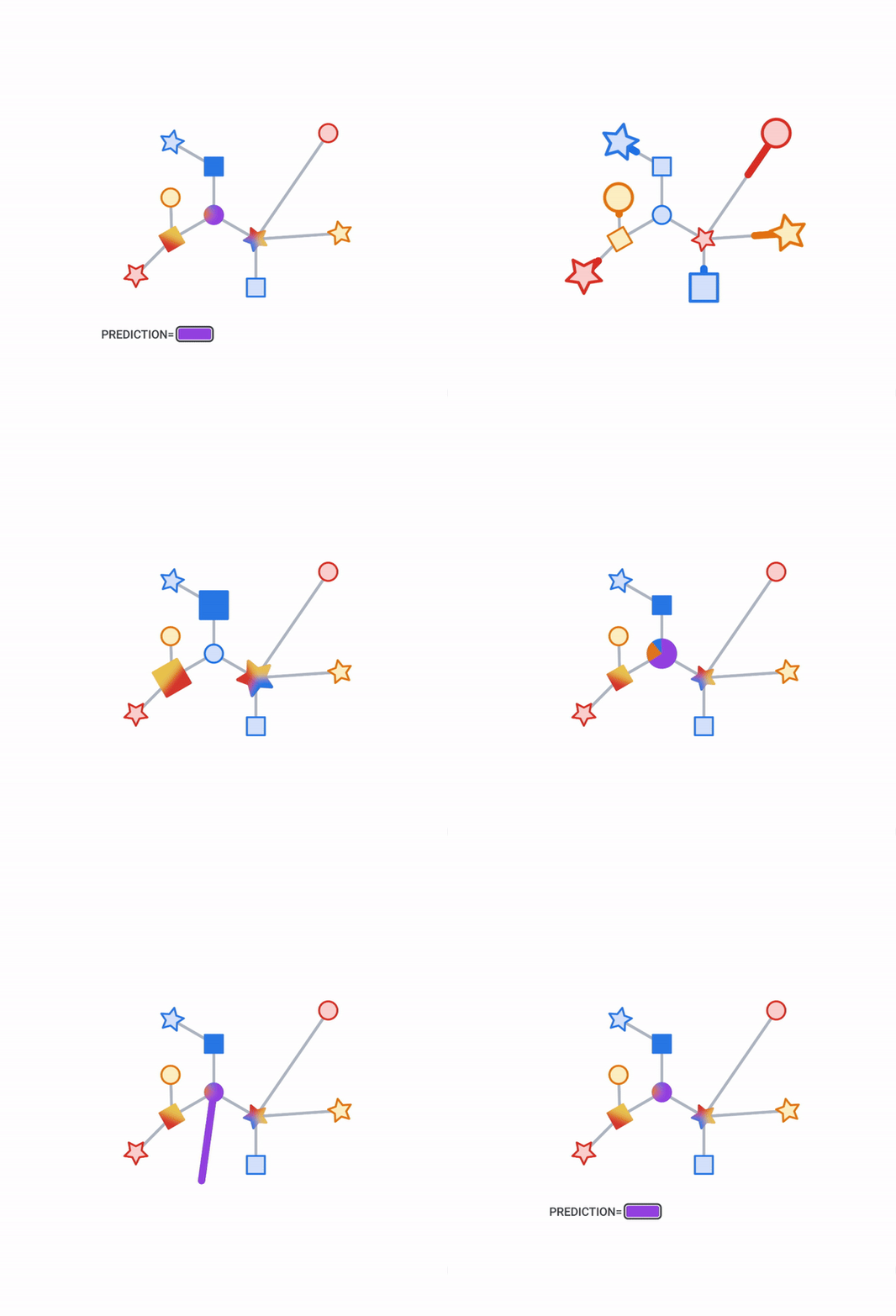
Graph Neural Networks (GNNs): Consider a graph \(G = \{V, E\}\) where \(V = \{v_1, v_2, \cdots, v_n\}\) and \(n = |V|\) is the number of nodes. Each node \(v_i\) has a feature vector \(x_i\). Modern GNNs update node representations iteratively by aggregating information from neighbours. The representation of node \(v_i\) at layer \(l\) is \(h^{(l)}_i\), with \(h_i^{(0)} = x_i\). The aggregation and combination at layer \(l\) are defined as: \(a_{i}^{(l)}=\text{AGGREGATE}^{(l)}\left(\left\{h_{j}^{(l-1)}: j \in \mathcal{N}(v_i)\right\}\right)\) \(h_{i}^{(l)}=\text{COMBINE}^{(l)}\left(h_{i}^{(l-1)}, a_{i}^{(l)}\right)\) where \(\mathcal{N}(v_i)\) is the set of first or higher-order neighbours of \(v_i\). Common aggregation functions include MEAN, MAX, and SUM. The COMBINE function fuses neighbor information into the node representation.
-
Graph Level Representation (READOUT): In general, a READOUT function is any function of the final-layer node representations from a GNN that we can use as a graph-level representation. So \(h_G = \text{READOUT}(\{h_i^{(L)}\})\) is a graph-level representation. A MEAN-READOUT is a simple example of a READOUT function, where the graph-level representation is the mean of the node representations.
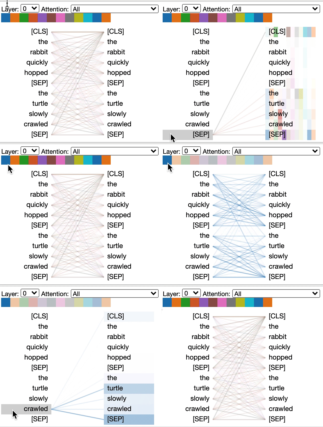
- Transformer: The Transformer architecture comprises layers with two main components: a self-attention module and a position-wise feed-forward network (FFN). Let \(H = [h_1^\top, \cdots, h_n^\top]^\top\in ℝ^{n\times d}\) be the input to the self-attention module, where \(d\) is the hidden dimension and \(h_i\in ℝ^{1\times d}\) is the hidden representation at position \(i\). The input \(H\) is projected using matrices \(W_Q\inℝ^{d\times d_K}, W_K\inℝ^{d\times d_K}\), and \(W_V\inℝ^{d\times d_V}\) to obtain representations \(Q, K, V\). Self-attention is computed as: \(Q = HW_Q,\ K = HW_K,\ V = HW_V,\ A = \frac{QK^\top}{\sqrt{d_K}},\ Attn(H) = \text{softmax}(A)V\) where \(A\) captures the similarity between queries and keys. This self-attention mechanism allows the model to understand relevant information in the sequence comprehensively.
Graphormer
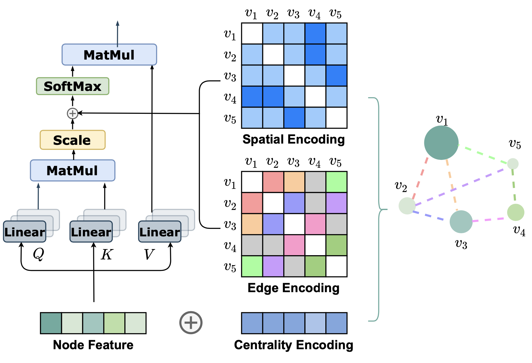
Centrality Encoding
In a sequence modelling task, Attention captures the semantic correlations between the nodes (tokens). The goal of this encoding is to capture the most important nodes in the graph. This is important information as important (heavily connected) nodes affect Let’s take an example. Say we want to compare airports and find which one is the largest. We need a common metric to compare them, so we take the sum of the total daily incoming and outgoing flights, giving us the busiest airports. This is what the algorithm is doing logically to identify the ‘busiest’ nodes. Similarly, these learnable vectors help the model to flag these important nodes in the graph. All this culminates in better performance for graph-based tasks such as molecule generation.
This is the Centrality Encoding equation, given as:
\[h_{i}^{(0)} = x_{i} + z^{-}_{deg^{-}(v_{i})} + z^{+}_{deg^{+}(v_{i})}\]Let’s analyse this term by term:
- \(h_{i}^{(0)}\) - Representation (\(h\)) of vertice i (\(v_{i}\)) at the 0th layer (first input)
- \(x_{i}\) - Feature vector of vertice i (\(v_{i}\))
- \(z^{-}_{deg^{-}(v_{i})}\) - Learnable embedding vector (\(z\)) of the indegree (\(deg^{-}\)) of vertice i (\(v_{i}\))
- \(z^{+}_{deg^{+}(v_{i})}\) - Learnable embedding vector (\(z\)) of the outdegree (\(deg^{+}\)) of vertice i (\(v_{i}\))
This is an excerpt of the code used to compute the Centrality Encoding
self.in_degree_encoder = nn.Embedding(num_in_degree, hidden_dim, padding_idx=0)
self.out_degree_encoder = nn.Embedding(num_out_degree, hidden_dim, padding_idx=0)
# Intial node feature computation.
node_feature = (node_feature + self.in_degree_encoder(in_degree) + self.out_degree_encoder(out_degree))
Spatial Encoding
There are several methods for encoding the position information of the tokens in a sequence. In a graph, however, there is a problem. Graphs consist of nodes (analogous to tokens) connected with edges in a non-linear, multi-dimensional space. There’s no inherent notion of an “ordering” or a “sequence” in its structure, but as with positional information, it’ll be helpful if we inject some sort of structural information when we process the graph.
The authors propose a novel encoding called Spatial Encoding. Take a pair of nodes (analogous to tokens) as input and output a scalar value as a function, \(\phi(v_i, v_j)\). The authors choose \(\phi(v_i, v_j)\) to be shortest path distance (SPD) between the nodes. This scalar value is then added to the element corresponding to the operation between the two nodes in the Query-Key product matrix.
\[A_{ij} = \frac{(h_i W_Q)(h_j W_K)^T}{\sqrt{d}} + b_{\phi(v_i, v_j)}\]The above equation shows the modified computation of the Query-Key Product matrix. Notice that the additional term \(b_{\phi(v_i, v_j)}\), a learnable scalar value, is just an embedding look-up and acts like a bias term. Since this structural information is independent of which layer of our model is using it, we share this value across all layers.
The benefits of using such an encoding are:
- Our receptive field has effectively increased, as we are no longer limited to the information from our neighbours, as is what happens in conventional message-passing networks.
- The model determines the best way to adaptively attend to the structural information. For example, if the scalar valued function is a decreasing function for a given node, we know that the nodes closer to our node are more important than the ones farther away.
Edge Encoding
Graphormer’s edge encoding method significantly enhances the way the model incorporates structural features from graph edges into its attention mechanism. The prior approaches either add edge features to node features or use them during aggregation, propagating the edge information only to associated nodes. Graphormer’s approach ensures that edges play a vital role in the overall node correlation.
Initially, node features \((h_i, h_j)\) and edge features \((x_{e_n})\) from the shortest path between nodes are processed. For each pair of nodes \((v_i, v_j)\), the edge features on the shortest path \(SP_{ij}\) are averaged after being weighted by learnable embeddings \((w^E_n)\), this results in the edge encoding \(c_{ij}\):
\[c_{ij} = \frac{1}{N} \sum_{n=1}^{N} x_{e_n} (w^E_n)^T\]This is then incorporated as the edge features into the attention score between nodes via a bias-like term. After incorporating the edge and spatial encodings, the value of \(A_{ij}\) is now:
\[A_{ij} = \frac{(h_i W_Q)(h_j W_K)^T}{\sqrt{d}} + b_{\phi(v_i,v_j)} + c_{ij}\]This ensures that edge features directly contribute to the attention score between any two nodes, allowing for a more nuanced and comprehensive utilization of edge information. The impact is significant, and it greatly improves the performance, as proven empirically in the Experiments section.
VNode
The [VNode] (or a Virtual Node) is arguably one of the most important contributions from the work. It is an artificial node that is connected to all other nodes. The authors cite this paper
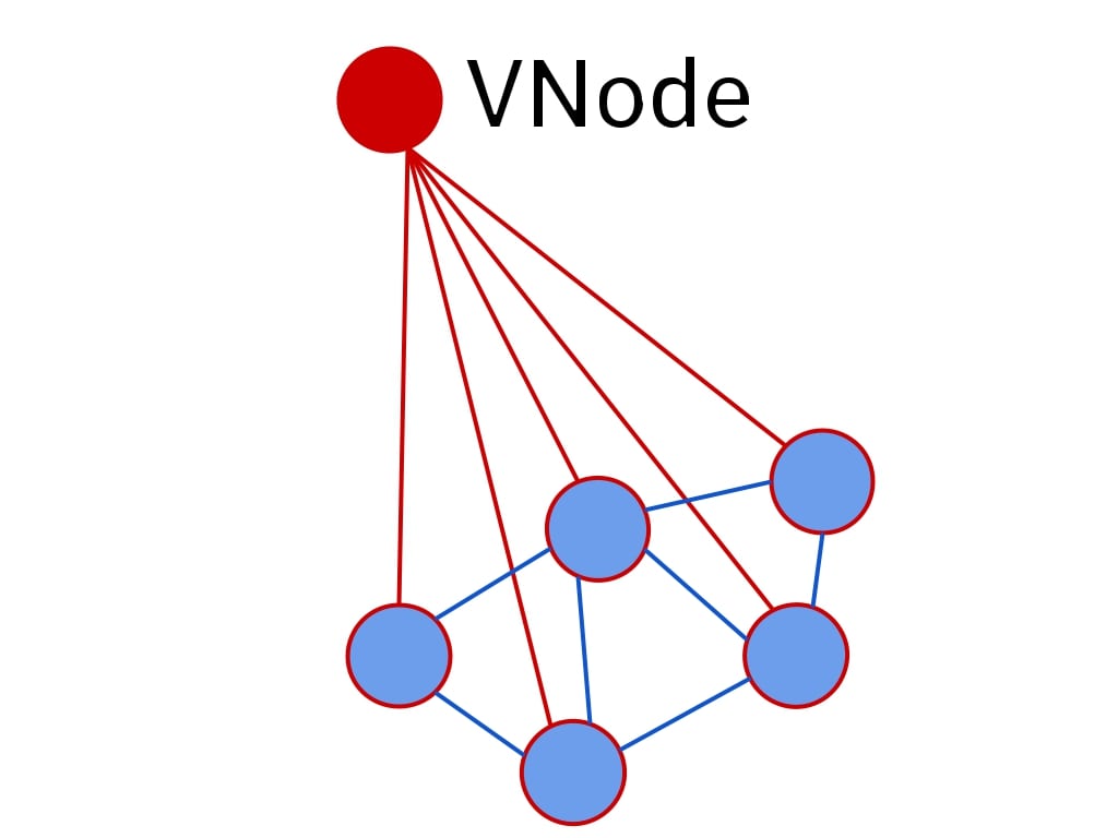
However, since this is not a physical connection, \(b_{\phi([VNode], v)}\) is set to be a distinct learnable vector (for all \(v\)) to provide the model with this important geometric information.
[CLS] (introduced in
More about [CLS] tokens
In implementation, NLP models have a distinct learnable embedding vector (along with other token embeddings in the mebedding matrix) and append this to the start of every training example, and the final layer representation of this token is used for the task (e.g. sentiment analysis, harmful-ness prediction, etc.). With enough task-specific (downstream) data the [CLS] token can learn to extract task-relevant information from the data, without having to train the model again!
With graphs and text being different modalities, the [VNode] also helps in relaying global information to distant or non-connected clusters in a graph. This is significantly important to the model’s expressivity, as this information might otherwise never propagate. In fact, the [VNode] becomes a learnable and dataset-specific READOUT function.
This can be implemented as follows:
    # Initialize the VNode
    self.v_node = nn.Embedding(1, num_heads)
    ...
    # During forward pass (suppose VNode is the first node)
    ...
    headed_emb = self.v_node.weight.view(1, self.num_heads, 1)
    graph_attn[:, :, 1:, 0] = graph_attn[:, :, 1:, 0] + headed_emb
        #(n_graph, n_heads, n_nodes + 1, n_nodes + 1)
    graph_attn[:, :, 0, :] = graph_attn[:, :, 0, :] + headed_emb
    ...
The design choice of one [VNode] per head enables each head to encode different global information.
Theoretical aspects of expressivity
These are the three main facts from the paper,
- With appropriate weights and \(\phi\), GCN
, GraphSAGE , and GIN are all special cases of a Graphormer. - Graphormer is better than architectures that are limited by the 1-WL test. (so all traditional GNNs!)
- With appropriate weights, every node representation in the output can be MEAN-READOUT.
The spatial encoding provides the model with important geometric information. Observe that with an appropriate \(b_{\phi(v_i, v_j)}\), the model can find (learn) neighbours for any \(v_i\) and thus easily implement mean-statistics (GCN!). By knowing the degree (some form of centrality encoding), mean-statistics can be transformed into sum-statistics; it (indirectly) follows that various statistics can be learned by different heads, which leads to varied representations and allows GraphSAGE, GIN or GCN to be modeled as a Graphormer. We also provide explicit mathematical equations on how the above claims can be realized, feel free to skip them.
Proof(s) for Fact 1
For each type of aggregation, we provide simple function and weight definitions that achieve it,
- Mean Aggregate :
- Set \(b_{\phi(v_i, v_j)} = 0\) when \(\phi(v_i, v_j) = 1\) and \(-\infty\) otherwise,
- Set \(W_Q = 0, W_K = 0\) and let \(W_V = I\) (Identity matrix), using these,
- \[h^{(l)}_{v_i} = \sum_{v_j \in N(v_i)} softmax(A_{ij}) * (W_v * h^{(l-1)}_{v_j}) \implies h^{(l)}_{v_i} = \frac{1}{|N(v_i)|}*\sum_{v_j \in N(v_i)} h^{(l-1)}_{v_j}\]
- Sum Aggregate :
- For this, we just need to get the mean aggregate and then multiply by \(\|N(v_i)\|\),
- Loosely, the degree can be extracted from centrality-encoding by an attention head, and then the FFN can multiply this to the learned mean aggregate, the latter part is a direct consequence of the universal approximation theorem.
- Max Aggregate :
- For this one we assume that if we have \(t\) dimensions in our hidden state, we also have t heads.
- The proof is such that each Head will extract the maximum from neighbours, clearly, to only keep immediate neighbours around, we can use the same formulation for \(b\) and \(\phi\) as in the mean aggregate.
- Using \(W_K = e_t\) (t-th unit vector), \(W_K = e_t\) and \(W_Q = 0\) (Identity matrix), we can get a pretty good approximation to the max aggregate. To get the full deal however, we need a hard-max instead of the soft-max being used; to accomplish this we finally consider the bias in the query layer (i.e., something like
nn.Linear(in_dim, out_dim, use_bias=True)), set it to \(T \cdot I\) with a high enough \(T\) (temperature), this will make the soft-max behave like a hard-max.
Fact 2 follows from Fact 1, with GIN being the most powerful traditional GNN, which can theoretically identify all graphs distinguishable by the 1-WL test, as it is now a special case of Graphormer. The latter can do the same (& more!).
The WL Test and an example for Fact 2
First we need to fix some notation for the WL test. Briefly, the formulation can be expressed as -
\[c^{(k+1)}(v) = HASH(c^{(k)}(v), \{c^{(k)}(u)\}_{u \in N(v)} )\]where \(c^{(k)}(v)\) is the \(k^{th}\) iteration representation (color for convenience) of node \(v\) and importantly \(HASH\) is an injective hash function. Additionally, all nodes with the same color have the same feature vector
Given this, consider the following graphs -
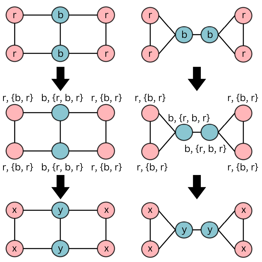
The hashing process converges in one iteration itself, now the 1-WL test would count number of colors and that vector would act as the final graph representation, which for both of the graphs will be \([0, 0, 4, 2]\) (i.e., \([count(a), count(b), count(x), count(y)]\)), even though they are different, the 1-WL test fails to distinguish them. There are several such cases and thus it can be said traditional GNNs are fairly limited in their expressivity.
However for the graphormer, Shortest Path Distances (SPD) directly affects attention weights (because the paper uses SPD as \(\phi(v_i, v_j)\)), and if we look at the SPD sets for the two types of nodes (red and blue) in both the graphs, (we have ordered according to the BFS traversal by top left red node, though any ordering would suffice)
- Left graph -
- Red nodes - \(\{ 0, 1, 1, 2, 2, 3 \}\)
- Blue nodes - \(\{1, 0, 2, 1, 1, 2\}\)
- Right graph -
- Red nodes - \(\{0, 1, 1, 2, 3, 3\}\)
- Blue nodes - \(\{1, 0, 1, 1, 2, 2\}\)
What is important is not that red and blue nodes have a different SPD set, but that these two types of nodes have different SPD sets across the two graphs. This signal can help the model distinguish the two graphs and is the reason why Graphormer is better than 1-WL test limited architectures.
More importantly, Fact 3 implies that Graphormer allows the flow of Global (and Local) information within the network. This truly sets the network apart from traditional GNNs, which can only aggregate local information up to a fixed radius (or depth).
Traditional GNNs are designed to prevent this type of flow, as with their architecture, this would lead to over-smoothening. However, the clever design around [VNode] prevents this from happening in Graphormer. The addition of a supernode along with Attention and the learnable \(b_{\phi(v_i, v_j)}\) facilitate this, the [VNode] can relay global information, and the attention mechanism can selectively choose from there.
Over-smoothening
Over-smoothening results in traditional GNNs when the neighbourhood considered for feature aggregation is too large. If we build a 10 layer deep network for a graph where the maximum distance bwteen any two nodes is 10, then all nodes will aggregate information from all other nodes, and the final representation will be the same for all nodes. Thus näively adding a [VNode] / Super Node would lead to over-smoothening in traditional GNNs.
Operations such as MEAN_READOUT involve aggregation over all nodes, making it a global operation. Given that Fact 3 implies that every node representation can be MEAN-READOUT, this means that the model can learn to selectively propagate global information using the [VNode].
Proof for Fact 3
Setting \(W_Q = W_K = 0\), and the bias terms in both to be \(T \cdot 1\) (where T is temperature), as well as, setting \(W_V = I\) (Identity matrix), with a large enough \(T\) (much larger than the scale of \(b_{\phi(v_i, v_j)}\), so that \(T^2 1 1^T\) can dominate), we can get MEAN-READOUT on all nodes. Note that while this proof doesn’t require [VNode], it should be noted that, the [Vnode] is very important to establish a balance between this completely global flow and the local flow. As in a normal setting, with the \(T\) not being too large, the only way for global information is through the [VNode], as the \(b_{\phi(v_i, v_j)}\) would most likely limit information from nodes that are very far.
Experiments
The researchers conducted comprehensive experiments to evaluate Graphormer’s performance against state-of-the-art models like GCN
Two variants of Graphormer, Graphormer (L=12, d=768) and a smaller GraphormerSMALL (L=6, d=512), were evaluated on the OGB-LSC quantum chemistry regression challenge (PCQM4M-LSC), one of the largest graph-level prediction dataset with over 3.8 million graphs.
The results, as shown in Table 1, demonstrate Graphormer’s significant performance improvements over previous top-performing models such as GIN-VN, DeeperGCN-VN, and GT.
Table 1: Results on PCQM4M-LSC
| Model | Parameters | Train MAE | Validate MAE |
|---|---|---|---|
| GIN-VN | 6.7M | 0.1150 | 0.1395 |
| DeeperGCN-VN | 25.5M | 0.1059 | 0.1398 |
| GT | 0.6M | 0.0944 | 0.1400 |
| GT-Wide | 83.2M | 0.0955 | 0.1408 |
| GraphormerSMALL | 12.5M | 0.0778 | 0.1264 |
| Graphormer | 47.1M | 0.0582 | 0.1234 |
Notably, As pointed out in the VNode section, Graphormer does not encounter over-smoothing issues, with both training and validation errors continuing to decrease as model depth and width increased. Additionally, Graph Transformer (GT) showed no performance gain despite a significant increase in parameters from GT to GT-Wide, highlighting Graphormer’s scaling capabilities. We also observe a strong overfitting (>0.045 difference between train and validate MAE) for Transformer based models. This can be attributed to its special structure, as it can extract more information from the training data.
Graph Trasformer (GT)
The Graph Transformer is an architecture which works on heterogeneous graphs. It uses a transformer to create several graphs at runtime by combining several meta-paths and the using a traditional GNN to aggregate information. As a transformer is not involved in the information relay stage, it’s expressivity is mid-way between a traditional GNN and a Graphormer.
Further experiments for graph-level prediction tasks were performed on datasets from popular leaderboards like OGBG (MolPCBA, MolHIV) and benchmarking-GNNs (ZINC), which also showed Graphormer consistently outperforming top-performing GNNs.
By using the ensemble with ExpC
Comparison against State-of-the-Art Molecular Representation Models
Let’s first take a look at GROVER
The authors further fine-tune GROVER on MolHIV and MolPCBA to achieve competitive performance along with supplying additional molecular features such as morgan fingerprints and other 2D features. Note that the Random Forest model fitted on these features alone outperforms the GNN model, showing the huge boost in performance granted by the same.
Table 2: Comparison between Graphormer and GROVER on MolHIV
| Method | # param. | AUC (%) |
|---|---|---|
| Morgan Finger Prints + Random Forest | 230K | 80.60±0.10 |
| GROVER | 48.8M | 79.33±0.09 |
| GROVER (LARGE) | 107.7M | 80.32±0.14 |
| Graphormer-FLAG | 47.0M | 80.51±0.53 |
However, as evident in Table 2, Graphormer manages to offer competitive performance on the benchmarks without even using the additional features (known to boost performance), which showcases it increases the expressiveness of complex information. Additionally the gap in performance can be attributed to the MolHIV dataset, which is too small for Graphormer to extract generalizable features.
Conclusion
Graphormer presents a novel way of applying Transformers to graph representation using the three structural encodings. While it has demonstrated strong performance across various benchmark datasets, significant progress has been made since the original paper. Structure-Aware Transformer