Accelerating Equivariant Graph Neural Networks with JAX
A Tutorial on How to Make EGNNs Faster
Introduction
This blogpost serves as a tutorial for the fast and scalable training of Equivariant Neural Networks, which are slower to train due to the handling of more complex data. We propose leveraging JAX’s capabilities to address these challenges. In this work, we analyze the benefits of utilizing JAX and provide a detailed breakdown of the steps needed to achieve a fully JIT-compatible framework. This approach not only enhances the performance of Neural Networks but also opens the door for future research in developing fully equivariant transformers using JAX. The code used in this tutorial is available here.
This blogpost serves three purposes:
- Explain the ideas of equivariance in networks while also explaining some of the methods used.
- Give an overview of the performance tests conducted on the two approaches.
- Provide an overview of reproduction results for the Equivariant Graph Neural Network.
Recap of Equivariance
As equivariance is prevalent in the natural sciences
Following these works, more efficient implementations have emerged, with the first being the Equivariant Graph Neural Network (EGNN)
More recently, transformer architectures have been utilized within the field of equivariant models. While not typically used for these types of problems due to how they were originally developed for sequential tasks
Equivariant Graph Neural Networks
Given a set of \(T_g\) transformations on a set \(X\) (\(T_g: X \rightarrow X\)) for an element \(g \in G\), where \(G\) is a group acting on \(X\), a function \(\varphi: X \rightarrow Y\) is equivariant to \(g\) iff an equivalent transformation \(S_g: Y \rightarrow Y\) exists on its output space \(Y\), such that:
In other words, translating the input set \(T_g(x)\) and then applying \(\varphi(T_x(x))\) on it yields the same result as first running the function \(y = \varphi(x)\) and then applying an equivalent translation to the output \(S_g(y)\) such that Equation 1 is fulfilled and \(\varphi(x+g) = \varphi(x) + g\)
Equivariant Graph Neural Networks
For a given graph \(\mathcal{G} = (\mathcal{V}, \mathcal{E})\) with nodes \(v_i \in \mathcal{V}\) and edges \(=e_{ij} \in \mathcal{E}\), we can define a graph convolutional layer as the following:
where \(\mathbf{h}\_i^l \in \mathbb{R}^{nf}\) is the nf-dimensional embedding of node \(v_i\) at layer \(l\), \(a_{ij}\) are the edge attributes, \(\mathcal{N}\_i\) is the set of neighbors of node \(v_i\), and \(\varphi_e\) and \(\varphi_h\) are the edge and node operations respectively, typically approximated by Multilayer Perceptrons (MLPs).
To make this implementation equivariant,
This idea of using the distances during computation forms an important basis in these architectures, as it is a simple yet effective way to impose geometric equivariance within a system.
Why JAX?
JAX is a high-performance numerical computing library that provides several advantages over traditional frameworks. By default, JAX automatically compiles library calls using just-in-time (JIT) compilation, ensuring optimal execution. It utilizes XLA-optimized kernels, allowing for sophisticated algorithm expression without leaving Python. Furthermore, JAX also excels in utilizing multiple GPU or TPU cores and automatically evaluating gradients through differentiation transformations, making it ideal for high-compute scenarios.
This is partially caused by how JAX often uses pointers to reference elements in memory instead of copying them, which has several advantages:
- Efficiency: Through pointers, JAX avoids the unnecessary copying of data, resulting in faster computations and lower memory usage.
- Functionally Pure: Since JAX functions are pure (i.e., contain no side effects), using pointers ensures that the data is not accidentally modified, maintaining the integrity of all operations.
- Automatic Differentiation: JAX’s efficient gradient computation relies on its functional programming model. Pointers allow JAX to track operations and dependencies without data duplication.
Experiments
N-Body dataset
In this dataset, a dynamical system consisting of 5 atoms is modeled in 3D space. Each atom has a positive and negative charge, a starting position and a starting velocity. The task is to predict the position of the particles after 1000 time steps. The movement of the particles follow the rules of physics: Same charges repel and different charges attract. The task is equivariant in the sense, that translating and rotating the 5-body system on the input space is the same as rotating the output space.
QM9 dataset
This dataset consists of small molecules and the task is to predict a chemical property. The atoms of the molecules have 3 dimensional positions and each atom is one hot encoded to the atom type. This task is an invariant task, since the chemical property does not depend on position or rotation of the molecule. In addition, larger batch sizes were also experimented with due to smaller sizes causing bottlenecks during training.
Data Preparation
Here, we introduce a straightforward method for preprocessing data from a PyTorch-compatible format to one suitable for JAX. Our approach handles node features, edge attributes, indices, positions, and target properties. The key step would be converting the data to jax numpy (jnp) arrays, ensuring compatibility with JAX operations. For usage examples, refer to qm9\utils.py or n_body\utils.py.
Training
We now address the key differences and steps in adapting the training loop, model saving, and evalution functions for JAX (refer to main_qm9.py and nbody_egnn_trainer.py).
JAX uses a functional approach to define and update the model parameters. We use jax.jit via the partial decorator for JIT compilation, which ensures that our code runs efficiently by compiling the functions once and then executing them multiple times. We also utilize static_argnames as decorators for the loss and update functions, which specify the arguments to treat as static. By doing this, JAX can assume these arguments will not change and optimize the function accordingly.
Moreover, model initialization in JAX requires knowing the input sizes beforehand. We extract features to get their shapes and initialize the model using model.init(jax_seed, *init_feat, max_num_nodes). This seed initializes the random number generators, which then produces the random number sequences used in virtually all processes. Also, this seed is created using the jax.random.PRNGKey function, which is used for all random operations. This ensures that they are all reproducible and can be split into multiple independent keys if needed.
The loss function is called through jax.grad(loss_fn)(params, x, edge_attr, edge_index, pos, node_mask, edge_mask, max_num_nodes, target). jax.grad is a powerful tool in JAX for automatic differentiation, allowing us to compute gradients of scalar-valued functions with respect to their inputs.
Evaluation
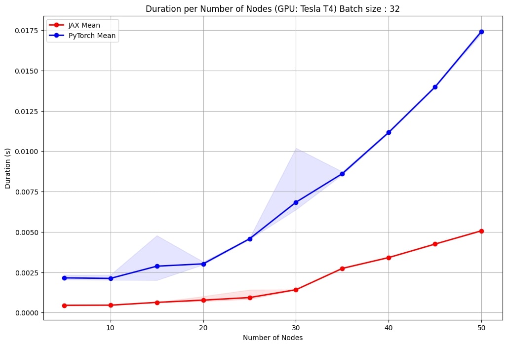
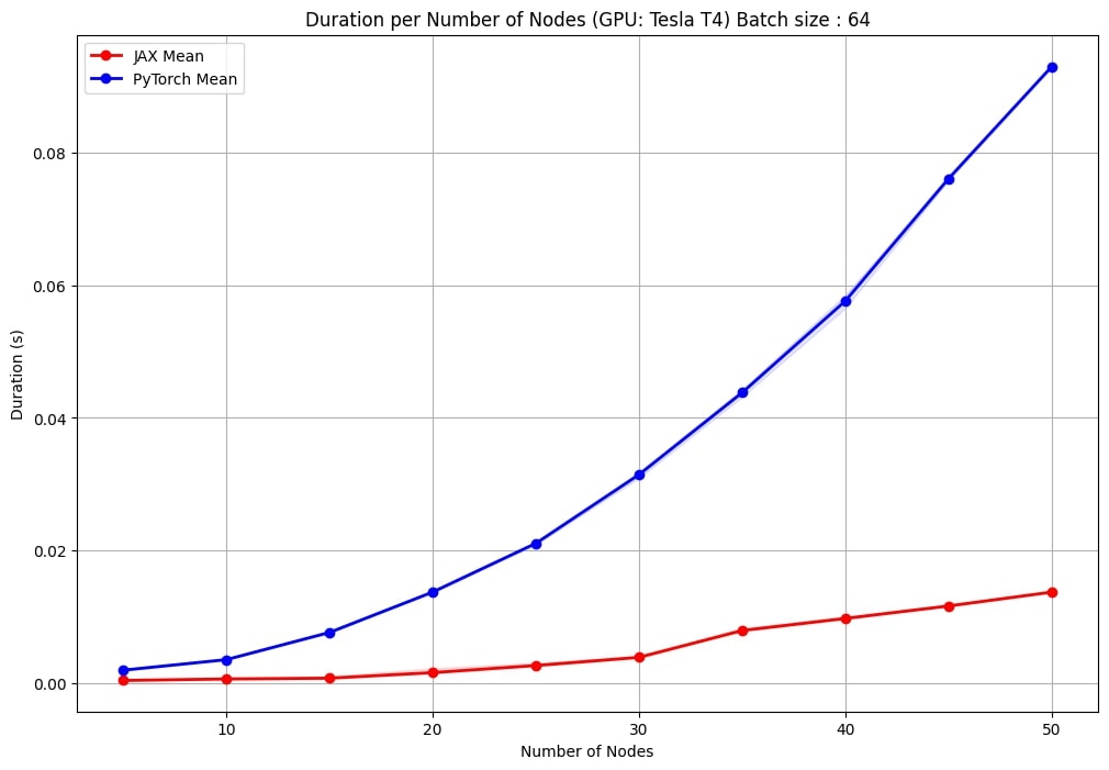
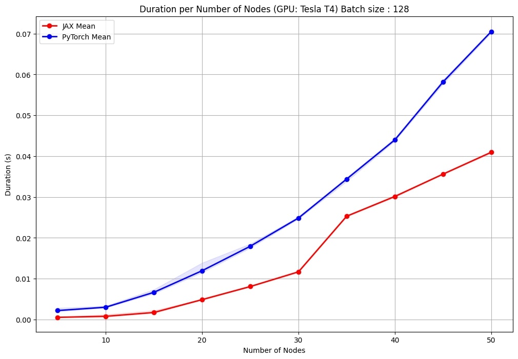
Speed Comparison
The EGNN authors


One notable observation is the consistency in performance. The JAX implementation exhibits less variance in duration values, resulting in more stable and predictable performances across runs. This is particularly important for large-scale applications where the performance consistency can impact overall system reliability and efficiency.
Additionally, as the number of nodes increases, the JAX implementation maintains a less steep increase in computation time compared to PyTorch. This indicates better scalability, making the JAX-based EGNN more suitable for handling larger and more complex graphs.
Reproduction Results
To show that our implementation generally preserves the performance and characteristics of the base model, we perform a reproduction of the results reported in
| Task | EGNN | EGNN (Ours) |
|---|---|---|
| QM9 (εHOMO) (meV) | 29 | 75 |
| N-Body (Position MSE) | 0.0071 | 0.0025 |
Table 1. Reproduction results comparing
Here, our EGNN implementation outperforms the original author’s implementation on the N-Body dataset. Moreover, other publicly available EGNN implementations also achieve a similar performance as our model on our data. We therefore argue that the increased performance stems from how the dataset is generated slightly differently compared to the one presented in
Concluding Remarks
Our EGNN comparisons reveal that the JAX-based model is faster than traditional PyTorch implementations, benefiting from JIT compilation to optimize runtime performance. In addition, we also demonstrate that these JAX-based models also achieve comparable performances to the aforementioned PyTorch ones, meaning that they are generally more suitable for equivariance tasks.
We also adapted the model for two well-known datasets: the QM9 dataset for molecule property prediction and the N-body dataset for simulating physical systems. This demonstrates the flexibility and potential of our JAX framework as a strong foundation for further development. Our work suggests that the JAX-based EGNN framework can be effectively extended to other applications, facilitating future research and advancements in equivariant neural networks and beyond.
You can find the code to our experiments here.